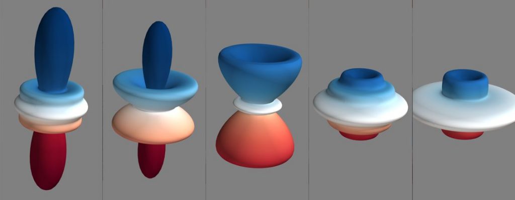
Attached below is a Python script to display spherical harmonics and spherical harmonic superpositions. Spherical harmonics are the angular wavefunctions (“eigenfunctions”) used to describe rotational states of molecules and the angular properties of electrons in atoms (i.e., “atomic orbitals”). A single eigenfunction of the Schrödinger equation is time-independent but dynamics can be described by a superposition (sum) of eigenfunctions. E.g., the square of a sum of spherical harmonics predicts the angular orientation of a molecule as function of time.

To use the script, you need to have a functional version of Python running on your computer. The header describes how to set up the correct environment using Anaconda Python. Have fun and comment if you found any issues or want to share your experience.

# PHYSICAL BACKGROUND
# -------------------
# This Python code plots a superposition of spherical harmonics (angular
# wave functions), that correspond to the energy eigenstates of a rotating 
# molecule or to the angular wavefunction of the electron in the hydrogen atom.
# The square of the angular angular wavefunction describes the probability to 
# observe the particle at the corresponding angle.
# Note that each eigenfunction is a time-independent solution to the angular 
# Schrödinger equation. "Add" additional eigenfunctions with different J and m 
# quantum numbers s to create a state superposition ("wave packet"), which 
# describes time-dependent properties, such as pseudo-classical molecular rotation.
#
# RUNNING THE CODE
#---------------------------------------------------------------------------
# To run Mayavi in Conda, it is necessary to create an environment for 
# Python 3.6 (or lower) including numpy, scipy and pyqtgraph. It is neccessary 
# to install VTK and Mayavi via PIP ("conda install" does not work).
# I use Anaconda Python [download from: https://conda.io/miniconda.html]
# In an administrator Conda shell, run:
# > conda create -n mayavi python=3.6 pyqt=5
# > conda activate mayavi
# > conda install numpy scipy pyqtgraph ipython
# > pip install vtk
# > pip install mayavi
# It is required to activate the (mayavi) environment (line 2) each time when 
# opening a new shell. Return to your (base) shell with "conda activate base".
#
# To run the script, I suggest you open an ipython shell and copy/paste the 
# code in three batches (marked [1],[2], and [3]). Note that only wavefunctions 
# with quantum numbers m = -J...J are allowed. In a conda shell, type:
# > conda activate mayavi
# > ipython
# and start copy/pasting the code from below.
#
# Written by Thomas Schultz, Apr. 2021
# Feel free to use and modify the code according to the Creative Commons license 
# [see: https://creativecommons.org/licenses/by/4.0/]
#---------------------------------------------------------------------------

#-----------------------------------------------------------------#
# [1a] Import mathematical functions and define wave functions ---#
#-----------------------------------------------------------------#
from numpy import sin, cos, pi, exp, mgrid
from scipy.special import sph_harm

# The rotational wavefunctions are the Spherical Harmonics. 
# For explicit ways to calculate the angular wavefunctions, refer to a textbook.
def TiWf (J,m,theta,phi):               # Time-independent angular wave function  
    return sph_harm(m, J, theta, phi)

def TdWf(k,t,phase):                    # Time dependent wave function. WF(r,t) = TiWf(r) * TdWf(t)
    return np.exp(-1j*k*(t+phase))      # k is the wavevector (angular frequency), == T(J,B)/2*pi

# To look at time-dependent wavefunctions, we need the state energies / terms
B = 3.27e9                              # Rotational constant for CS2 (in Hz) 
def EJ(J): return J*(J+1)               # Energy of a J state in a rigid linear rotor
def T(J,B): return B*J*(J+1)            # Energy term of J state (in freq. units)

#-----------------------------------------------------------#
# [1b] Plot a time-independent wave function             ---#
#-----------------------------------------------------------#
from mayavi import mlab
      
# Spatial coordinates for plotting:
# Create a grid over a sphere defined by r, phi, theta
# More grid points look better, but take more time to calculate
r = 0.3         # radius
grid = 80j
phi, theta = mgrid[0:pi:grid, 0:2*pi:2*grid]

# Spherical to Cartesian coordinate transformation
x = r * sin(phi) * cos(theta)
y = r * sin(phi) * sin(theta)
z = r * cos(phi)    

SqWF = abs(TiWf(2,1,theta,phi))**2      # Wave function psi-squared for state J=2, m=1
plot = mlab.mesh(SqWF *x, SqWF *y, SqWF *z, colormap='RdBu', opacity=1., transparent=True)

#--------------------------------------------------------------------------#
# [2a] Initialize a list of wavefunctions to plot a state superposition ---#
#--------------------------------------------------------------------------#

t = 0; deltaT = 5e-12                   # Initial time (0), time-increment (1 ps)
J = [0,]                                # List of J-values
m = [0,]                                # List of m-values
Amp = [1.,]                             # List of amplitudes
phase = np.array([0.,])                 # List of initial phases
showReal = [True,]                      # Show the real or imaginary part
showImag = [True,]                      # ... of the wavefunction
TiWfList = []                           # Initialize list of time-independent wavefunctions (don't recalculate for each step)
kList = []                              # Initialize list of k-vectors for propagation
for _J,_m,_a in zip(J,m,Amp):           # Calculate TiWf for each state in the list. (recalculate when J, m, Amp change)
    TiWfList.append(_a* TiWf(_J,_m,theta,phi))  # Time-independent wavefunctions WF(r)
    kList.append(T(_J,B))               # k-vectors for WF propagation: WF(r,t) = WF(r)*exp(-ikt)

#----------------------------------------------------------------------#
# [2b] Animated plot: Update TiWf*TdWf for incrementing time values ---#
#----------------------------------------------------------------------#

@mlab.animate(delay=200)
def anim():
    global TiWfList, kList, phase, t, deltaT, x,y,z
    while True:
        if showReal[0] and showImag[0]:
            sumWF = TiWfList[0]*TdWf(kList[0],t,phase[0])
        else: 
          if showReal[0]:
            sumWF = (TiWfList[0]*TdWf(kList[0],t,phase[0])).real +(0+0j)
          if showImag[0]:
            sumWF = (TiWfList[0]*TdWf(kList[0],t,phase[0])).imag +(0+0j)
          if not (showReal[0]) and not (showImag[0]):
            sumWF = (TiWfList[0]*TdWf(kList[0],t,phase[0])).imag *(0+0j)
        if len(kList)>1: 
          for i in range(len(kList)-1):
            if (showReal[i+1] and showImag[i+1]):
              sumWF += TiWfList[i+1]*TdWf(kList[i+1],t,phase[i+1])
            elif showReal[i+1]:
              sumWF += ((TiWfList[i+1]*TdWf(kList[i+1],t,phase[i+1])).real +(0+0j))
            elif showImag[i+1]:
              sumWF += ((TiWfList[i+1]*TdWf(kList[i+1],t,phase[i+1])).imag +(0+0j))
        plot.mlab_source.x = np.absolute(sumWF)**2 *x       # replace x data
        plot.mlab_source.y = np.absolute(sumWF)**2 *y       # replace y data
        plot.mlab_source.z = np.absolute(sumWF)**2 *z       # replace z data
        yield
        t += deltaT                           # increment time 
anim()

#---------------------------------------------------------------#
# [3a] Create a user interface for easy control of the plot. ---#
#--- I use a PyQt ParameterTree as user interface            ---#
#---------------------------------------------------------------#    
import pyqtgraph as pg
from pyqtgraph.Qt import QtCore, QtGui, QtWidgets
import pyqtgraph.parametertree.parameterTypes as pTypes
from pyqtgraph.parametertree import Parameter, ParameterTree, ParameterItem, registerParameterType
QtCore.QCoreApplication.setAttribute(QtCore.Qt.AA_ShareOpenGLContexts)
qt_app = QtWidgets.QApplication(sys.argv)

# List of parameters for each state
rotParameters = [
        {'name': 'amplitude', 'type': 'float', 'value': 1, 'limits': (0, 1), 'default': 1.},
        {'name': 'J', 'type': 'int', 'value': 0, 'limits': (0, 100)},
        {'name': 'm', 'type': 'int', 'value': 0, 'limits': (0, 100)},
        {'name': 'phase', 'type': 'float', 'value': 0., 'default': 0.},
        {'name': 'Show real**2', 'type': 'bool', 'value': True, 'tip': "add abs(real(phi)) to plot"}, 
        {'name': 'Show imag**2', 'type': 'bool', 'value': True, 'tip': "add abs(imag(phi)) to plot"}, 
              ]

# This class allows the user to add new parameters into the parameter tree
class ScalableGroup(pTypes.GroupParameter):
    """ Extendable group of parameters for parameter tree."""
    def __init__(self, **opts):
        opts['type'] = 'group'
        opts['addText'] = "Add"
        opts['addList'] = ['State']
        pTypes.GroupParameter.__init__(self, **opts)
        self.counter = 1
        self.addChild(dict(name="State %d" %(self.counter), children=rotParameters, removable=True, renamable=True))
    def addNew(self, typ):
        self.addChild(dict(name="State %d" %(self.counter+1), children=rotParameters, removable=True, renamable=True))
        self.counter += 1

# List of global property parameters 
parameters = [ 
    {'name': 'Global Properties', 'type': 'group', 'expanded': True, 'children': [
        {'name': 'Radius', 'type': 'float', 'value': 0.3, 'limits': (0.001, 10), 'default': 0.3, 'tip': "radius of image"},
#        {'name': 'Animate', 'type': 'bool', 'value': False, 'tip': "animate plot"},
        {'name': 'Speed (ps)', 'type': 'float', 'value': 10, 'limits': (0.01, 200), 'default': 0.5, 'tip': "time step for animation"},
        ]},
    ScalableGroup(name="Rotational State Properties"),  # Call the ScalableGroup to add rotational parameters to the tree
]

# If anything changes in the parameter tree, update the wavefunction parameters
def change(parameterTree, changes):
    """ This function must handle all user requests by interpreting the 
        parameter origin, name, and value"""
    global B, Amp, J, m, phase, TiWfList, kList, showReal, showImag, theta, phi, deltaT, x,y,z
    for parameterName, change, data in changes:
        path = parameterTree.childPath(parameterName)
        print(f'path: {path}')
        if path is not None:
            childName = '.'.join(path)
        else:
            childName = parameterName.name()
        if change == "childAdded": 
            print("== child added ==")            # New state added: Now update all wavefunctions
            Amp, J, m, phase, TiWfList, kList, showReal, showImag = updateWaveFunctions(parameterTree)  
        if change == "value":                     # Value change: Update only the affected wavefunction
          if path[0] == 'Rotational State Properties':
            stateNo = int(path[1].split()[1])-1
            parameter = path[2]
            print(f'state: {stateNo};   parameter: {parameter} = {data}')
            if parameter == 'amplitude': Amp[stateNo] = float(data)
            if parameter == 'J': J[stateNo] = int(data)
            if parameter == 'm': m[stateNo] = int(data)
            if parameter == 'phase': phase[stateNo] = float(data)
            if parameter == 'Show real**2': showReal[stateNo] = float(data)
            if parameter == 'Show imag**2': showImag[stateNo] = float(data)
            TiWfList[stateNo] = Amp[stateNo]* TiWf(J[stateNo],m[stateNo],theta,phi)
            kList[stateNo] = T(J[stateNo],B)
          elif path[0] == 'Global Properties':    # Global property change: update the affected parameters
            parameter = path[1]
            if parameter == 'Speed (ps)': deltaT = data*1e-12; 
            if parameter == 'Radius': 
              r = data
              x = r * sin(phi) * cos(theta)
              y = r * sin(phi) * sin(theta)
              z = r * cos(phi)

# This recalculates the whole list of wavefunctions. 
def updateWaveFunctions(p):
    global B, theta, phi
    Amp,J,m,phase,TiWfList,kList,showReal,showImag = [],[],[],[],[],[],[],[]
    values = p.getValues()["Rotational State Properties"][1]  # Table values for States
    for state in list(values):
        data = values[state][1]
        _a = float(data['amplitude'][0])
        Amp.append(_a)
        _j = data['J'][0]
        J.append(_j)
        _m = data['m'][0]
        m.append(_m)
        _p = float(data['phase'][0]) 
        phase.append(_p)
        _real = data['Show real**2'][0]
        showReal.append(_real)
        _imag = data['Show imag**2'][0]
        showImag.append(_imag)
        TiWfList.append(_a* TiWf(_j,_m,theta,phi))
        kList.append(T(_j,B))
    return Amp,J,m,phase,TiWfList,kList,showReal,showImag

#Now we actually create a window and show the parameter tree
win = QtGui.QWidget()
win.resize(280,500)
layout = QtGui.QGridLayout()
win.setLayout(layout)
p = Parameter.create(name='params', type='group', children=parameters)
p.sigTreeStateChanged.connect(change)
tree = ParameterTree()
tree.setParameters(p, showTop=False)
tree.setWindowTitle('Angular states')
layout.addWidget(tree)
win.show()